Evaluation of automatic annotations

This notebook demonstrates automatic annotation model evaluation.

First, load the required libraries.

import json

from matplotlib import pyplot as plt
from matplotlib import mlab
import numpy as np
from scipy.stats import gaussian_kde

Next, load the validation data

validation_file = "data/validation.test.json"
validation_file_all = "data/validation.all.json"
validation_file_train = "data/validation.train.json"

with open(validation_file, "r") as f:
    validation = json.load(f)

with open(validation_file_all, "r") as f:
    validation_all = json.load(f)

with open(validation_file_train, "r") as f:
    validation_train = json.load(f)

list(validation.keys())

['ious',
 'polyline_hausdorff_distances',
 'length_differences',
 'true_positives',
 'false_positives',
 'false_negatives']

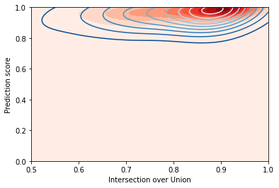
Plot the Scores vs. Intersection over Union Density. A good model will show a peak in the top-right corner, have a high mean IoU, and show similar results for the full set and the test set.

fig = plt.figure()

ax = fig.add_subplot(
    111,
    xlabel="Intersection over Union",
    ylabel="Prediction score",
)

iou_X, iou_Y = np.mgrid[0.5:1.:100j, 0.:1.:100j]
iou_positions = np.vstack([iou_X.ravel(), iou_Y.ravel()])

# All images
ious_all, iou_scores_all = zip(*validation_all["ious"])
ious_all = np.array(ious_all)
iou_scores_all = np.array(iou_scores_all)

iou_kernel_all = gaussian_kde(np.vstack([ious_all, iou_scores_all]))
iou_values_all = np.reshape(iou_kernel_all(iou_positions).T, iou_X.shape)

p = ax.contourf(
    iou_X,
    iou_Y,
    iou_values_all,
    levels=10,
    cmap="Reds",
)

# Test set
ious, iou_scores = zip(*validation["ious"])
ious = np.array(ious)
iou_scores = np.array(iou_scores)

iou_kernel = gaussian_kde(np.vstack([ious, iou_scores]))
iou_values = np.reshape(iou_kernel(iou_positions).T, iou_X.shape)

p = ax.contour(
    iou_X,
    iou_Y,
    iou_values,
    levels=10,
    cmap="Blues_r",
)

print("mean IoU:")
print(f"Full set: {np.mean(ious_all)}")
print(f"Test set: {np.mean(ious)}")

mean IoU:
Full set: 0.8135264456997439
Test set: 0.8054630747838181

p.levels

array([ 0. ,  1.5,  3. ,  4.5,  6. ,  7.5,  9. , 10.5, 12. , 13.5, 15. ])

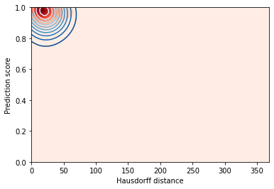
Plot the Scores vs. Hausdorff Distance Density. A good model will show a peak in the top-left corner, have a low mean Hausdorff Distance, and show similar results for the full set and the test set.

fig = plt.figure()

ax = fig.add_subplot(
    111,
    xlabel="Hausdorff distance",
    ylabel="Prediction score",
)

# All images
phds_all, phd_scores_all = zip(*validation_all["polyline_hausdorff_distances"])
phds_all = np.array(phds_all)
phd_scores_all = np.array(phd_scores_all)

# Test set
phds, phd_scores = zip(*validation["polyline_hausdorff_distances"])
phds = np.array(phds)
phd_scores = np.array(phd_scores)

max_phd = max(phds_all.max(), phds.max())

phd_X, phd_Y = np.mgrid[0.:max_phd:100j, 0.:1.:100j]
phd_positions = np.vstack([phd_X.ravel(), phd_Y.ravel()])

# All images
phd_kernel_all = gaussian_kde(np.vstack([phds_all, phd_scores_all]))
phd_values_all = np.reshape(phd_kernel_all(phd_positions).T, phd_X.shape)

p = ax.contourf(
    phd_X,
    phd_Y,
    phd_values_all,
    levels=10,
    cmap="Reds",
)

# Test set
phd_kernel = gaussian_kde(np.vstack([phds, phd_scores]))
phd_values = np.reshape(phd_kernel(phd_positions).T, phd_X.shape)

p = ax.contour(
    phd_X,
    phd_Y,
    phd_values,
    levels=10,
    cmap="Blues_r",
)

print("mean Hausdorff distance:")
print(f"Full set: {np.mean(phds_all)}")
print(f"Test set: {np.mean(phds)}")

mean Hausdorff distance:
Full set: 29.224007981876568
Test set: 28.76616770267623

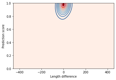
Plot the Scores vs. Length Difference Density. A good model will show a peak in the top-centre, have a low mean and standard deviation of length difference, and show similar results for the full set and the test set.

fig = plt.figure()

ax = fig.add_subplot(
    111,
    xlabel="Length difference",
    ylabel="Prediction score",
)

# All images
l_diffs_all, l_diff_scores_all = zip(*validation_all["length_differences"])
l_diffs_all = np.array(l_diffs_all)
l_diff_scores_all = np.array(l_diff_scores_all)

# Test set
l_diffs, l_diff_scores = zip(*validation["length_differences"])
l_diffs = np.array(l_diffs)
l_diff_scores = np.array(l_diff_scores)

max_l_diff = max(np.abs(l_diffs_all).max(), np.abs(l_diffs).max())

l_diff_X, l_diff_Y = np.mgrid[-max_l_diff:max_l_diff:100j, 0.:1.:100j]
l_diff_positions = np.vstack([l_diff_X.ravel(), l_diff_Y.ravel()])

# All images
l_diff_kernel_all = gaussian_kde(np.vstack([l_diffs_all, l_diff_scores_all]))
l_diff_values_all = np.reshape(l_diff_kernel_all(l_diff_positions).T, l_diff_X.shape)

p = ax.contourf(
    l_diff_X,
    l_diff_Y,
    l_diff_values_all,
    levels=10,
    cmap="Reds",
)

# Test set
l_diff_kernel = gaussian_kde(np.vstack([l_diffs, l_diff_scores]))
l_diff_values = np.reshape(l_diff_kernel(l_diff_positions).T, l_diff_X.shape)

p = ax.contour(
    l_diff_X,
    l_diff_Y,
    l_diff_values,
    levels=10,
    cmap="Blues_r",
)

print("mean length difference:")
print(f"Full set: {np.mean(l_diffs_all)}")
print(f"Test set: {np.mean(l_diffs)}")

print("mean absolute length difference:")
print(f"Full set: {np.mean(np.abs(l_diffs_all))}")
print(f"Test set: {np.mean(np.abs(l_diffs))}")

print("std length difference:")
print(f"Full set: {np.std(l_diffs_all)}")
print(f"Test set: {np.std(l_diffs)}")

mean length difference:
Full set: -3.308262066472856
Test set: 5.155644178390503
mean absolute length difference:
Full set: 28.52835982924359
Test set: 28.5195529460907
std length difference:
Full set: 46.44938175547716
Test set: 51.003080907488574

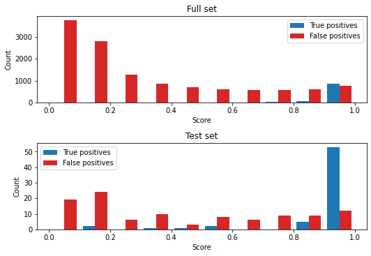
Plot the score histograms for true positives and false positives. A good model will have a peak in true positives close to 1 and lower scores for false positives.

fig = plt.figure(
    figsize=(7.5, 5.2),
    tight_layout=True,
)
ax = fig.add_subplot(
    211,
    xlabel="Score",
    ylabel="Count",
    title="Full set",
)


h, b, p = ax.hist(
    [validation_all["true_positives"], validation_all["false_positives"]],
    bins=np.linspace(0., 1., num=11),
    label=["True positives", "False positives"],
    color=["tab:blue", "tab:red"],
)
ax.legend()

ax = fig.add_subplot(
    212,
    xlabel="Score",
    ylabel="Count",
    title="Test set",
)


h, b, p = ax.hist(
    [validation["true_positives"], validation["false_positives"]],
    bins=np.linspace(0., 1., num=11),
    label=["True positives", "False positives"],
    color=["tab:blue", "tab:red"],
)
ax.legend()

print("Full set:")
print(f'True positives:  {len(validation_all["true_positives"]):4d}')
print(f'False positives: {len(validation_all["false_positives"]):4d}')
print(f'False negatives: {validation_all["false_negatives"]:4d}')

print("\nTest set:")
print(f'True positives:  {len(validation["true_positives"]):4d}')
print(f'False positives: {len(validation["false_positives"]):4d}')
print(f'False negatives: {validation["false_negatives"]:4d}')

Full set:
True positives:   997
False positives: 12522
False negatives:  422

Test set:
True positives:    64
False positives:  106
False negatives:   25

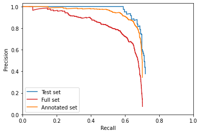
Plot Precision vs. Recall and calculate average precision for the full set, and the test set

# Full set
true_positives_all = np.array(validation_all["true_positives"])
false_positives_all = np.array(validation_all["false_positives"])
false_negatives_all = validation_all["false_negatives"]

precision_all = [0.]
recall_all = [1.]

for score_cutoff in np.sort(np.concatenate((true_positives_all, false_positives_all))):
    tp = np.count_nonzero(true_positives_all >= score_cutoff)
    fp = np.count_nonzero(false_positives_all >= score_cutoff)
    try:
        pr = tp / (tp + fp)
        re = tp / (tp + false_negatives_all)
    except ZeroDivisionError:
        pass
    finally:
        precision_all.append(pr)
        recall_all.append(re)

precision_all.append(1.)
recall_all.append(0.)

precision_all = np.array(precision_all)
recall_all = np.array(recall_all)

ap_precision_values_all = []
for ap_recall_value in np.linspace(0., 1., num=11, endpoint=True):
    ap_precision_values_all.append(precision_all[recall_all >= ap_recall_value].max())

average_precision_all = sum(ap_precision_values_all) / len(ap_precision_values_all)

# Test set
true_positives = np.array(validation["true_positives"])
false_positives = np.array(validation["false_positives"])
false_negatives = validation["false_negatives"]

precision = [0.]
recall = [1.]

for score_cutoff in np.sort(np.concatenate((true_positives, false_positives))):
    tp = np.count_nonzero(true_positives >= score_cutoff)
    fp = np.count_nonzero(false_positives >= score_cutoff)
    try:
        pr = tp / (tp + fp)
        re = tp / (tp + false_negatives)
    except ZeroDivisionError:
        pass
    finally:
        precision.append(pr)
        recall.append(re)

precision.append(1.)
recall.append(0.)

precision = np.array(precision)
recall = np.array(recall)

ap_precision_values = []
for ap_recall_value in np.linspace(0., 1., num=11, endpoint=True):
    ap_precision_values.append(precision[recall >= ap_recall_value].max())

average_precision = sum(ap_precision_values) / len(ap_precision_values)

# Annotated only
true_positives_train = np.array(validation_train["true_positives"])
false_positives_train = np.array(validation_train["false_positives"])
false_negatives_train = validation_train["false_negatives"]

precision_train = [0.]
recall_train = [1.]

for score_cutoff in np.sort(np.concatenate((true_positives_train, false_positives_train))):
    tp = np.count_nonzero(true_positives_train >= score_cutoff)
    fp = np.count_nonzero(false_positives_train >= score_cutoff)
    try:
        pr = tp / (tp + fp)
        re = tp / (tp + false_negatives_train)
    except ZeroDivisionError:
        pass
    finally:
        precision_train.append(pr)
        recall_train.append(re)

precision_train.append(1.)
recall_train.append(0.)

precision_train = np.array(precision_train)
recall_train = np.array(recall_train)

ap_precision_values_train = []
for ap_recall_value in np.linspace(0., 1., num=11, endpoint=True):
    ap_precision_values_train.append(precision_train[recall_train >= ap_recall_value].max())

average_precision_train = sum(ap_precision_values_train) / len(ap_precision_values_train)

fig = plt.figure()
ax = fig.add_subplot(
    111,
    xlabel="Recall",
    ylabel="Precision",
    xlim=(0., 1.),
    ylim=(0., 1.03),
)
ax.plot(recall[1:-1], precision[1:-1], c="tab:blue", label="Test set")
ax.plot(recall_all[1:-1], precision_all[1:-1], c="tab:red", label="Full set")
ax.plot(recall_train[1:-1], precision_train[1:-1], c="tab:orange", label="Annotated set")
ax.legend()

print("AP_50:")
print(f"Full set: {average_precision_all}")
print(f"Test set: {average_precision}")
print(f"Training set: {average_precision_train}")

AP_50:
Full set: 0.5879457315920177
Test set: 0.6866600298656048
Training set: 0.6683919288386905

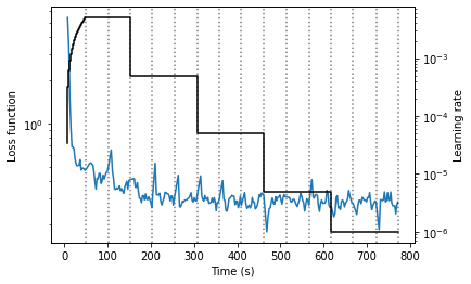
We also want to visualise the training process

from training_log_parser import parse_lines

with open("data/20210809_14_model_log.txt", "r") as f:
    epochs = parse_lines(f)

all_vals = {}
for epoch in epochs:
    for key in epoch.keys():
        all_vals.setdefault(key, []).extend(epoch[key])

t = np.cumsum(all_vals["time"])
fig = plt.figure()
ax = fig.add_subplot(
    111,
    xlabel="Time (s)",
    yscale="log",
)
ax.set_ylabel("Loss function")

tot_t = 0.
for epoch in epochs[:-1]:
    tot_t += sum(epoch["time"])
    ax.axvline(tot_t, c="k", ls="dotted", alpha=0.5)


ax.plot(t, all_vals["loss"], label="loss")

tot_t += sum(epochs[-1]["time"])
ax.axvline(tot_t, c="k", ls="dotted", label="epoch", alpha=0.5)

#ax.legend()

ax2 = ax.twinx()
ax2.set_yscale("log")
ax2.set_ylabel("Learning rate")
ax2.plot(t, all_vals["lr"], c="k", label="Learning rate", ds="steps-pre")
#ax2.legend()

[<matplotlib.lines.Line2D at 0x7f5b8ec93cd0>]

Putting together one figure

def get_quantiles(values):
    """
    converts values to quantiles

    Parameters
    ----------

    values: array
        evenly spaced kde estimate values

    Returns
    -------

    quantiles: array of shape values.shape
        can be passed to plt.contour to produce quantile contour plot

    to_value: callable
        takes a quantile as an argument and converts to value
    """
    sort_indices = np.unravel_index(np.argsort(values, axis=None), values.shape)
    sorted_values = values[sort_indices]
    integral = np.cumsum(sorted_values) / sorted_values.sum()

    quantiles = np.empty_like(values)
    quantiles[sort_indices] = integral

    def to_value(quant):
        return sorted_values[np.nonzero(integral >= quant)[0][0]]

    return quantiles, to_value

fontdict={"fontweight": "bold"}
tloc = "right"
ty = 0
cmap_all = "Reds"
cmap = "Blues_r"
c_all = "tab:red"
c = "tab:blue"
quantiles = np.array([0.25, 0.5, 0.75, 0.9, 1.])
quantiles_all = np.array([0.15, 0.25, 0.5, 0.75, 0.9, 1.])

iou_xlabel = "Intersection over Union"
phd_xlabel = "Hausdorff Distance (px)"
l_diff_xlabel = "Length Difference (px)"

iou_title = "(b) "
phd_title = "(c) "
l_diff_title = "(d) "
pr_title = "(e) "

fig_width = 180  # mm
fig_width /= 25.4  # inches
fig_height = fig_width

fig = plt.figure(
    figsize=(fig_width, fig_height),
    tight_layout=True,
)

t = np.cumsum(all_vals["time"])
ax = fig.add_subplot(
    311,
    xlabel="Training time (s)",
    yscale="log",
)
ax.set_ylabel("Loss function")
ax.set_title(
    "(a) ",
    fontdict=fontdict,
    loc=tloc,
    y=0.85,
)

tot_t = 0.
for epoch in epochs[:-1]:
    tot_t += sum(epoch["time"])
    ax.axvline(tot_t, c="k", ls="dotted", alpha=0.5)


ax.plot(t, all_vals["loss"], c="k", label="loss")

tot_t += sum(epochs[-1]["time"])
ax.axvline(tot_t, ymax=0.85, c="k", ls="dotted", label="epoch", alpha=0.5)

#ax.legend()

ax2 = ax.twinx()
ax2.set_yscale("log")
ax2.set_ylabel("Learning rate")
ax2.plot(t, all_vals["lr"], c="g", label="Learning rate", ds="steps-pre")
#ax2.legend()

ax_loc = 322
for metric in ["iou", "phd", "l_diff"]:
    ax_loc += 1
    xlabel = locals()[f"{metric}_xlabel"]
    X = locals()[f"{metric}_X"]
    Y = locals()[f"{metric}_Y"]
    values_all = locals()[f"{metric}_values_all"]
    values = locals()[f"{metric}_values"]
    s_all = locals()[f"{metric}s_all"]
    s = locals()[f"{metric}s"]
    kernel_all = locals()[f"{metric}_kernel_all"]
    kernel = locals()[f"{metric}_kernel"]
    scores_all = locals()[f"{metric}_scores_all"]
    scores = locals()[f"{metric}_scores"]
    title = locals()[f"{metric}_title"]

    ax = fig.add_subplot(
        ax_loc,
        xlabel=xlabel,
        ylabel="Prediction score",
    )

    quantile_values, to_value = get_quantiles(values_all)
    p_all = ax.contourf(
        X,
        Y,
        quantile_values,
        levels=quantiles_all,
        cmap=cmap_all,
    )
    p_all_outlier_mask = kernel_all(np.vstack([s_all, scores_all])) < to_value(p_all.levels[0])
    o_all = ax.plot(
        s_all[p_all_outlier_mask],
        scores_all[p_all_outlier_mask],
        marker=".",
        ls="",
        c=c_all,
    )
    quantile_values, to_value = get_quantiles(values)
    p = ax.contour(
        X,
        Y,
        quantile_values,
        levels=quantiles,
        cmap=cmap,
        zorder=10,
    )
    p_outlier_mask = kernel(np.vstack([s, scores])) < to_value(p.levels[0])
    o = ax.plot(
        s[p_outlier_mask],
        scores[p_outlier_mask],
        marker=".",
        ls="",
        c=c,
    )
    t = ax.set_title(
        title,
        fontdict=fontdict,
        loc=tloc,
        y=ty,
    )

# Precision vs. Recall
ax4 = fig.add_subplot(
    ax_loc + 1,
    xlabel="Detection Recall",
    ylabel="Detection Precision",
    xlim=(0., 1.),
    ylim=(0., 1.03),
)
ax4.plot(
    recall_all[1:-1],
    precision_all[1:-1],
    c=c_all,
    label="Full set",
)
ax4.plot(
    recall[1:-1],
    precision[1:-1],
    c=c,
    label="Test set",
)
ax4.plot(
    recall_train[1:-1],
    precision_train[1:-1],
    c="tab:orange",
    label="Annotated set",
)
t4 = ax4.set_title(
    pr_title,
    fontdict=fontdict,
    loc=tloc,
    y=ty,
)

# Hacking together the contours figure legend
proxy = [plt.Rectangle((0, 0), 1, 1, fc=pc.get_facecolor()[0]) for pc in p_all.collections]
proxy = list(np.insert(proxy, range(2, len(p.collections) + 1), p.collections[:-1]))
labels = list(np.insert(quantiles_all[:-1], range(2, len(quantiles) + 1), quantiles[:-1]))
proxy.insert(1, plt.Rectangle((0, 0), 1, 1, fc="None")),
labels.insert(1, "")

proxy1 = [plt.Rectangle((0, 0), 1, 1, fc="None"), plt.Rectangle((0, 0), 1, 1, fc="None")]
#proxy1 = ["None", "None"]
labels1 = ["Full set quantile:", "Test set quantile:"]

proxy1.extend(proxy)
labels1.extend(labels)

leg = fig.legend(
    proxy1,
    labels1,
    loc="lower center",
    #title="Contour Quantile",
    ncol=len(quantiles_all),
    bbox_to_anchor=(0.5, -0.09),
    frameon=False,
    #markerfirst=False,
)

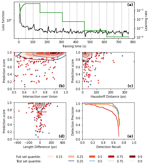
fig.savefig("autoannotation_evaluation_figure.pdf", dpi=600.0, bbox_inches="tight")