Flying insect activity-levels analysis

This notebook demonstrates analysis of flying insect activity levels data from camfi.

First, load the required libraries.

from datetime import datetime, timedelta, timezone
import itertools
import textwrap

from matplotlib import pyplot as plt
from matplotlib.ticker import MaxNLocator
import numpy as np
import pandas as pd
import scipy as sp
import statsmodels.api as sm
import statsmodels.formula.api as smf

from camfi.projectconfig import CamfiConfig
from camfi.plotting.matplotlib import (
    plot_activity_levels_summary,
    plot_activity_levels_summaries,
    plot_maelstroms_with_temperature,
)

Next, load the image metadata (including annotations from VIA). This file should have the corrected image capture timestamps (refer to the Wingbeat Analysis notebook).

config_path = "data/cabramurra_config.yml"

config = CamfiConfig.parse_yaml_file(config_path)

# We can print out our config using config.json() or config.yaml()
print(config.json(exclude_unset=True, indent=2))

{
  "root": "data",
  "via_project_file": "data/cabramurra_all_annotations.json",
  "day_zero": "2019-01-01",
  "output_tz": "+10:00",
  "filters": {
    "image_filters": {
      "min_annotations": 1
    }
  },
  "camera": {
    "camera_time_to_actual_time_ratio": 1.0,
    "line_rate": 90500.0
  },
  "time": {
    "camera_placements": {
      "2019-11_cabramurra/0004": {
        "camera_start_time": "2019-10-14T13:00:00+11:00",
        "actual_start_time": "2019-11-14T13:00:00+11:00",
        "location": "cabramurra"
      },
      "2019-11_cabramurra": {
        "camera_start_time": "2019-11-14T13:00:00+11:00",
        "location": "cabramurra"
      }
    }
  },
  "place": {
    "locations": [
      {
        "name": "cabramurra",
        "lat": -35.9507,
        "lon": 148.3972,
        "elevation_m": 1513.9,
        "tz": "+10:00"
      }
    ],
    "weather_stations": [
      {
        "location": {
          "name": "cabramurra_smhea_aws_072161",
          "lat": -35.94,
          "lon": 148.38,
          "elevation_m": 1482.4,
          "tz": "+10:00"
        },
        "data_file": "data/cabramurra_bom_weather_201911.csv"
      }
    ],
    "location_weather_station_mapping": {
      "cabramurra": "cabramurra_smhea_aws_072161"
    }
  },
  "wingbeat_extraction": {
    "device": "cpu",
    "scan_distance": 50
  },
  "annotator": {
    "crop": {
      "x0": 0,
      "y0": 0,
      "x1": 4608,
      "y1": 3312
    },
    "training": {
      "mask_maker": {
        "shape": [
          3312,
          4608
        ],
        "mask_dilate": 5
      },
      "min_annotations": 1,
      "max_annotations": 50,
      "test_set_file": "data/cabramurra_test_set.txt",
      "device": "cuda",
      "batch_size": 5,
      "num_workers": 2,
      "num_epochs": 15,
      "outdir": "data",
      "save_intermediate": true
    },
    "inference": {
      "output_path": "data/cabramurra_autoannotated.json",
      "device": "cuda",
      "backup_device": "cpu",
      "score_thresh": 0.0
    },
    "validation": {
      "autoannotated_via_project_file": "data/cabramurra_autoannotated.json",
      "image_sets": [
        "all",
        "test",
        "train"
      ],
      "output_dir": "data"
    }
  }
}

To get the timestamps for the images, we need to read the EXIF metadata from the image files. Here we also apply time correction. The code is commented out since the metadata has already been loaded into "data/cabramurra_all_annotations.json", but if you are working with a different dataset, or would like to re-run IO intensive this step, uncomment the code. This could also be achieved from the command-line interface to Camfi.

Note: It is assumed you have downloaded and extracted the images to "data/". Of course you can extract it elsewhere and change root config variable accordingly. The repository containing the images used in this example can be found here: https://doi.org/10.5281/zenodo.4950570.

# Uncomment if exif metadata hasn't been loaded already.
# config.load_all_exif_metadata()

After running the above two steps, you might like to save the results to a new VIA project file. Uncommenting the following will save a new VIA project file to "data/all_annotations_with_metadata.json".

# with open("data/all_annotations_with_metadata.json", "w") as f:
#     f.write(config.via_project.json(indent=2, exclude_unset=True))

For the following analyses, we need a Pandas DataFrame. The folowwing command builds a dataframe with an entry for each image, with data taken from sources specified in the config. We will also convert all the datetime_corrected values to AEST (+10:00, set in config file) - in our data they are in AEDT (+11:00).

df = config.get_merged_dataframe()
df

		img_key	filename	n_annotations	datetime_corrected	datetime_original	exposure_time	pixel_x_dimension	pixel_y_dimension	astronomical_twilight_start	nautical_twilight_start	...	maximum_wind_gust_time	temperature_9am_degC	relative_humidity_9am_pc	cloud_amount_9am_oktas	wind_direction_9am	wind_speed_9am_kph	temperature_3pm_degC	relative_humidity_3pm_pc	wind_direction_3pm	wind_speed_3pm_kph
location	date
cabramurra	2019-11-14	2019-11_cabramurra/0001/DSCF0001.JPG-1	2019-11_cabramurra/0001/DSCF0001.JPG	0	2019-11-14 18:00:03+10:00	2019-11-14 19:00:03	0.012048	4608	3456	2019-11-14 03:12:20.886936+10:00	2019-11-14 03:49:05.935004+10:00	...	23:04	4.9	95	3.0	W	17	10.1	73	W	22
	2019-11-14	2019-11_cabramurra/0001/DSCF0002.JPG-1	2019-11_cabramurra/0001/DSCF0002.JPG	0	2019-11-14 18:10:06+10:00	2019-11-14 19:10:06	0.009174	4608	3456	2019-11-14 03:12:20.886936+10:00	2019-11-14 03:49:05.935004+10:00	...	23:04	4.9	95	3.0	W	17	10.1	73	W	22
	2019-11-14	2019-11_cabramurra/0001/DSCF0003.JPG-1	2019-11_cabramurra/0001/DSCF0003.JPG	0	2019-11-14 18:20:09+10:00	2019-11-14 19:20:09	0.012048	4608	3456	2019-11-14 03:12:20.886936+10:00	2019-11-14 03:49:05.935004+10:00	...	23:04	4.9	95	3.0	W	17	10.1	73	W	22
	2019-11-14	2019-11_cabramurra/0001/DSCF0004.JPG-1	2019-11_cabramurra/0001/DSCF0004.JPG	0	2019-11-14 18:30:11+10:00	2019-11-14 19:30:11	0.020833	4608	3456	2019-11-14 03:12:20.886936+10:00	2019-11-14 03:49:05.935004+10:00	...	23:04	4.9	95	3.0	W	17	10.1	73	W	22
	2019-11-14	2019-11_cabramurra/0001/DSCF0005.JPG-1	2019-11_cabramurra/0001/DSCF0005.JPG	0	2019-11-14 18:40:14+10:00	2019-11-14 19:40:14	0.033333	4608	3456	2019-11-14 03:12:20.886936+10:00	2019-11-14 03:49:05.935004+10:00	...	23:04	4.9	95	3.0	W	17	10.1	73	W	22
	...	...	...	...	...	...	...	...	...	...	...	...	...	...	...	...	...	...	...	...	...	...
	2019-11-26	2019-11_cabramurra/0010/DSCF0860.JPG-1	2019-11_cabramurra/0010/DSCF0860.JPG	0	2019-11-26 05:13:26+10:00	2019-11-26 06:13:26	0.033333	4608	3456	2019-11-26 03:00:54.332543+10:00	2019-11-26 03:39:54.781647+10:00	...	13:34	13.6	55	8.0	NNW	41	3.1	99	WNW	35
	2019-11-26	2019-11_cabramurra/0010/DSCF0861.JPG-1	2019-11_cabramurra/0010/DSCF0861.JPG	0	2019-11-26 05:23:29+10:00	2019-11-26 06:23:29	0.033333	4608	3456	2019-11-26 03:00:54.332543+10:00	2019-11-26 03:39:54.781647+10:00	...	13:34	13.6	55	8.0	NNW	41	3.1	99	WNW	35
	2019-11-26	2019-11_cabramurra/0010/DSCF0862.JPG-1	2019-11_cabramurra/0010/DSCF0862.JPG	0	2019-11-26 05:33:31+10:00	2019-11-26 06:33:31	0.023810	4608	3456	2019-11-26 03:00:54.332543+10:00	2019-11-26 03:39:54.781647+10:00	...	13:34	13.6	55	8.0	NNW	41	3.1	99	WNW	35
	2019-11-26	2019-11_cabramurra/0010/DSCF0863.JPG-1	2019-11_cabramurra/0010/DSCF0863.JPG	0	2019-11-26 05:43:34+10:00	2019-11-26 06:43:34	0.018182	4608	3456	2019-11-26 03:00:54.332543+10:00	2019-11-26 03:39:54.781647+10:00	...	13:34	13.6	55	8.0	NNW	41	3.1	99	WNW	35
	2019-11-26	2019-11_cabramurra/0010/DSCF0864.JPG-1	2019-11_cabramurra/0010/DSCF0864.JPG	0	2019-11-26 05:53:37+10:00	2019-11-26 06:53:37	0.013889	4608	3456	2019-11-26 03:00:54.332543+10:00	2019-11-26 03:39:54.781647+10:00	...	13:34	13.6	55	8.0	NNW	41	3.1	99	WNW	35

8640 rows × 36 columns

To get a general overview of the activity levels observed throughout the study period, we pool the data from all cameras and plot the number of annotations per 10-minute interval:

# Setting frame of reference and
# adding a daynumber column to df, for simpler plots
df["daynumber"] = (
    df["datetime_corrected"] - config.timestamp_zero
).dt.total_seconds() / 86400

location_names = [location.name for location in config.place.locations]
fig = plot_activity_levels_summaries(
    df,
    location_names,
    x_column="daynumber",
    bin_width=10 / 1440,   # 10 minutes
    ax_kwargs=dict(
        ylabel="Number of annotations in 10 min bins",
        xlabel="Day Number"
    ),
    c="k",
)

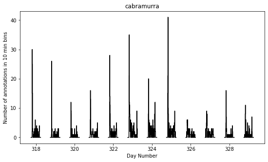
The gaps in the above figure are periods where the cameras were not set to take photos (they were only set to take photos between the hours of 19:00-07:00 AEDT each night).

There seems to be a periodic signal in the data, with more activity in the evening. We can take a closer look at this by pooling the data from all days into a single representative 24-hour period.

df["dayhour"] = (df["daynumber"] - np.floor(df["daynumber"])) * 24.

fig = plot_activity_levels_summaries(
    df,
    location_names,
    x_column="dayhour",
    bin_width=10 / 60,   # 10 minutes
    ax_kwargs=dict(
        ylabel="Number of annotations in 10 min bins",
        xlabel="Time of day (h)"
    ),
    c="k",
)

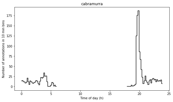
In the above figure we see a striking increase in activity levels during the hours of 19:20-20:20. This seems to be when the most insects are flying.

Instead of binning this data by absolute time of day, it would be nice to bin it according to the relative time from astronomical events, eg. sunset.

Here we calculate a “within_twilight” column, which is time after sunset, scaled to the duration of twilight. We’ll also calculate a “daylight_hours” column, which will be used later.

df["within_twilight"] = (
    df["datetime_corrected"] - df["sunset"]
) / (
    df["astronomical_twilight_end"] - df["sunset"]
)
df["daylight_hours"] = (df["sunset"] - df["sunrise"]).dt.total_seconds() / 3600

df

		img_key	filename	n_annotations	datetime_corrected	datetime_original	exposure_time	pixel_x_dimension	pixel_y_dimension	astronomical_twilight_start	nautical_twilight_start	...	wind_direction_9am	wind_speed_9am_kph	temperature_3pm_degC	relative_humidity_3pm_pc	wind_direction_3pm	wind_speed_3pm_kph	daynumber	dayhour	within_twilight	daylight_hours
location	date
cabramurra	2019-11-14	2019-11_cabramurra/0001/DSCF0001.JPG-1	2019-11_cabramurra/0001/DSCF0001.JPG	0	2019-11-14 18:00:03+10:00	2019-11-14 19:00:03	0.012048	4608	3456	2019-11-14 03:12:20.886936+10:00	2019-11-14 03:49:05.935004+10:00	...	W	17	10.1	73	W	22	317.750035	18.000833	-0.504471	13.978719
	2019-11-14	2019-11_cabramurra/0001/DSCF0002.JPG-1	2019-11_cabramurra/0001/DSCF0002.JPG	0	2019-11-14 18:10:06+10:00	2019-11-14 19:10:06	0.009174	4608	3456	2019-11-14 03:12:20.886936+10:00	2019-11-14 03:49:05.935004+10:00	...	W	17	10.1	73	W	22	317.757014	18.168333	-0.403632	13.978719
	2019-11-14	2019-11_cabramurra/0001/DSCF0003.JPG-1	2019-11_cabramurra/0001/DSCF0003.JPG	0	2019-11-14 18:20:09+10:00	2019-11-14 19:20:09	0.012048	4608	3456	2019-11-14 03:12:20.886936+10:00	2019-11-14 03:49:05.935004+10:00	...	W	17	10.1	73	W	22	317.763993	18.335833	-0.302793	13.978719
	2019-11-14	2019-11_cabramurra/0001/DSCF0004.JPG-1	2019-11_cabramurra/0001/DSCF0004.JPG	0	2019-11-14 18:30:11+10:00	2019-11-14 19:30:11	0.020833	4608	3456	2019-11-14 03:12:20.886936+10:00	2019-11-14 03:49:05.935004+10:00	...	W	17	10.1	73	W	22	317.770961	18.503056	-0.202121	13.978719
	2019-11-14	2019-11_cabramurra/0001/DSCF0005.JPG-1	2019-11_cabramurra/0001/DSCF0005.JPG	0	2019-11-14 18:40:14+10:00	2019-11-14 19:40:14	0.033333	4608	3456	2019-11-14 03:12:20.886936+10:00	2019-11-14 03:49:05.935004+10:00	...	W	17	10.1	73	W	22	317.777940	18.670556	-0.101282	13.978719
	...	...	...	...	...	...	...	...	...	...	...	...	...	...	...	...	...	...	...	...	...	...
	2019-11-26	2019-11_cabramurra/0010/DSCF0860.JPG-1	2019-11_cabramurra/0010/DSCF0860.JPG	0	2019-11-26 05:13:26+10:00	2019-11-26 06:13:26	0.033333	4608	3456	2019-11-26 03:00:54.332543+10:00	2019-11-26 03:39:54.781647+10:00	...	NNW	41	3.1	99	WNW	35	329.217662	5.223889	-7.947638	14.293727
	2019-11-26	2019-11_cabramurra/0010/DSCF0861.JPG-1	2019-11_cabramurra/0010/DSCF0861.JPG	0	2019-11-26 05:23:29+10:00	2019-11-26 06:23:29	0.033333	4608	3456	2019-11-26 03:00:54.332543+10:00	2019-11-26 03:39:54.781647+10:00	...	NNW	41	3.1	99	WNW	35	329.224641	5.391389	-7.851293	14.293727
	2019-11-26	2019-11_cabramurra/0010/DSCF0862.JPG-1	2019-11_cabramurra/0010/DSCF0862.JPG	0	2019-11-26 05:33:31+10:00	2019-11-26 06:33:31	0.023810	4608	3456	2019-11-26 03:00:54.332543+10:00	2019-11-26 03:39:54.781647+10:00	...	NNW	41	3.1	99	WNW	35	329.231609	5.558611	-7.755108	14.293727
	2019-11-26	2019-11_cabramurra/0010/DSCF0863.JPG-1	2019-11_cabramurra/0010/DSCF0863.JPG	0	2019-11-26 05:43:34+10:00	2019-11-26 06:43:34	0.018182	4608	3456	2019-11-26 03:00:54.332543+10:00	2019-11-26 03:39:54.781647+10:00	...	NNW	41	3.1	99	WNW	35	329.238588	5.726111	-7.658763	14.293727
	2019-11-26	2019-11_cabramurra/0010/DSCF0864.JPG-1	2019-11_cabramurra/0010/DSCF0864.JPG	0	2019-11-26 05:53:37+10:00	2019-11-26 06:53:37	0.013889	4608	3456	2019-11-26 03:00:54.332543+10:00	2019-11-26 03:39:54.781647+10:00	...	NNW	41	3.1	99	WNW	35	329.245567	5.893611	-7.562418	14.293727

8640 rows × 40 columns

We can now plot these data. This also plots a separate trace for each location (whereas the above plot only plots one trace for all the data).

fig = plot_activity_levels_summaries(
    df,
    location_names,
    x_column="within_twilight",
    bin_width=0.1,   # 10th of twilight duration
    ax_kwargs=dict(
        title="Plot of number of annotations relative to twilight",
        ylabel="Number of annotations",
        xlabel="Twilight durations since sunset"
    ),
    separate_plots=False,
    c="k",
)
twilight_vspan = fig.axes[0].axvspan(0, 1, alpha=0.3, label="Evening twilight")
legend = fig.axes[0].legend()

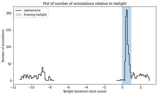
The moths appear to be flying during twilight. So lets select only those time points to quantify daily maelstrom intensity. Taking the sum of annotations during this period for each day, we can then look at how activity levels were across the days of the study period.

# We're only interested in the numeric columns
keep_dtypes = set(
    np.dtype("".join(t)) for t in itertools.product("ifu", "248")
)
keep_cols = filter(lambda c: df[c].dtype in keep_dtypes, df.columns)

# But even some of the numeric columns are irrelevant after aggregation
drop_cols = {
    "exposure_time",
    "pixel_x_dimension",
    "pixel_y_dimension",
    "dayhour",
    "within_twilight",
}
keep_cols = filter(lambda c: c not in drop_cols, keep_cols)

# For most of the columns, we just want to take the mean value
aggregation_functions = {column: (column, "mean") for column in keep_cols}

# But for "n_annotations", we want to take the sum
aggregation_functions["n_annotations"] = ("n_annotations", "sum")

# And we want to truncate "daynumber" to an integer
aggregation_functions["daynumber"] = ("daynumber", lambda x: int(x[0]))

# We also want to make a new column with the exposure (number of images
# taken) during each twilight interval.
aggregation_functions["exposures"] = ("n_annotations", "count")

# Now we select the data which was obtained during twilight,
# and group it by location and date, aggregating using the above-defined
# aggregation functions. This leaves us with a DataFrame with one row per
# date for each location in the study.
maelstrom_df = df[
    (df["within_twilight"] <= 1.) & (df["within_twilight"] >= 0)
].groupby(["location", "date"]).aggregate(**aggregation_functions)
maelstrom_df

		n_annotations	lat	lon	elevation_m	temperature_minimum_degC	temperature_minimum_evening_degC	temperature_maximum_degC	rainfall_mm	maximum_wind_gust_speed_kph	temperature_9am_degC	relative_humidity_9am_pc	cloud_amount_9am_oktas	wind_speed_9am_kph	temperature_3pm_degC	relative_humidity_3pm_pc	wind_speed_3pm_kph	daynumber	daylight_hours	exposures
location	date
cabramurra	2019-11-14	80	-35.9507	148.3972	1513.9	-0.6	4.7	12.3	0.0	41.0	4.9	95.0	3.0	17.0	10.1	73.0	22.0	317	13.978719	90
	2019-11-15	42	-35.9507	148.3972	1513.9	4.7	3.7	13.8	0.0	70.0	8.3	73.0	2.0	31.0	12.8	53.0	31.0	318	14.007941	100
	2019-11-16	35	-35.9507	148.3972	1513.9	3.7	3.3	14.3	0.0	48.0	5.9	69.0	NaN	11.0	13.2	35.0	20.0	319	14.036682	100
	2019-11-17	50	-35.9507	148.3972	1513.9	3.3	4.5	14.3	0.0	33.0	8.4	42.0	0.0	7.0	13.4	26.0	13.0	320	14.064925	100
	2019-11-18	79	-35.9507	148.3972	1513.9	4.5	7.5	16.0	0.0	43.0	7.6	45.0	2.0	15.0	14.5	35.0	24.0	321	14.092652	100
	2019-11-19	105	-35.9507	148.3972	1513.9	7.5	11.0	21.7	0.0	65.0	13.0	41.0	0.0	30.0	20.6	22.0	30.0	322	14.119846	100
	2019-11-20	59	-35.9507	148.3972	1513.9	11.0	15.0	23.1	0.0	31.0	15.0	31.0	1.0	7.0	21.3	23.0	17.0	323	14.146488	100
	2019-11-21	117	-35.9507	148.3972	1513.9	15.0	17.2	27.6	0.0	50.0	22.0	27.0	1.0	13.0	27.3	22.0	22.0	324	14.172561	100
	2019-11-22	33	-35.9507	148.3972	1513.9	17.2	11.3	22.6	0.0	54.0	19.8	34.0	1.0	15.0	21.7	39.0	26.0	325	14.198045	110
	2019-11-23	40	-35.9507	148.3972	1513.9	11.3	8.2	20.0	0.0	43.0	13.9	36.0	0.0	15.0	18.5	28.0	22.0	326	14.222923	110
	2019-11-24	43	-35.9507	148.3972	1513.9	8.2	11.8	19.8	0.0	41.0	13.0	60.0	0.0	9.0	18.2	40.0	22.0	327	14.247175	100
	2019-11-25	36	-35.9507	148.3972	1513.9	11.8	13.0	21.9	0.0	50.0	13.9	33.0	0.0	20.0	20.4	26.0	28.0	328	14.270782	100

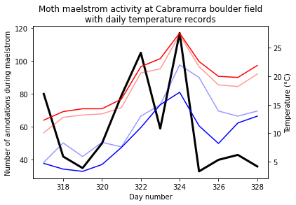
Now we can plot these data:

fig = plt.figure()
ax = fig.add_subplot(
    111,
    title="Moth maelstrom activity at Cabramurra boulder field\nwith daily temperature records",
    ylabel="Number of annotations during maelstrom",
    xlabel="Day number",
)
lines = plot_maelstroms_with_temperature(
    maelstrom_df,
    ax,
    maelstrom_kwargs=dict(
        c="k",
        lw=3,
    ),
)

We then may like to regress the activity levels against various factors. Given the activity level count data, we can proceed using a Poisson regression of n_annotations vs. the independent variables of interest.

First, we will select non-correlated covariates from maelstrom_df. Here we can add derived covariates, such as temperature_range and dewpoint_degC.

We also define a set drop of columns not to include as covariates.

maelstrom_df["temperature_range"] = maelstrom_df.temperature_maximum_degC - maelstrom_df.temperature_minimum_evening_degC
# maelstrom_df["dewpoint_3pm_degC"] = mpcalc.dewpoint_from_relative_humidity(
#     units.Quantity(maelstrom_df["temperature_3pm_degC"].array, "degC"),
#     units.Quantity(maelstrom_df["relative_humidity_3pm_pc"].array, "percent"),
# )

drop = {
    "n_annotations",           # Variable of interest
    "rainfall_mm",             # All zero in this dataset
    "cloud_amount_9am_oktas",  # Hass missing data
    "exposures",               # Exposure variable
    "lat",
    "lon",                     # All locations are the same
    "elevation_m",             # in this example
}
covariates = list(filter(lambda c: c not in drop, maelstrom_df.columns))

We can then plot scatter plots of all of the covariates.

grr = pd.plotting.scatter_matrix(
    maelstrom_df[["n_annotations", *covariates]],
    marker="o",
    figsize=(15, 15),
)
for ax in grr[-1, :]:
    ax.set_xlabel(ax.get_xlabel(), rotation=45, ha="right")
for ax in grr[:, 0]:
    ax.set_ylabel(ax.get_ylabel(), rotation=45, ha="right")

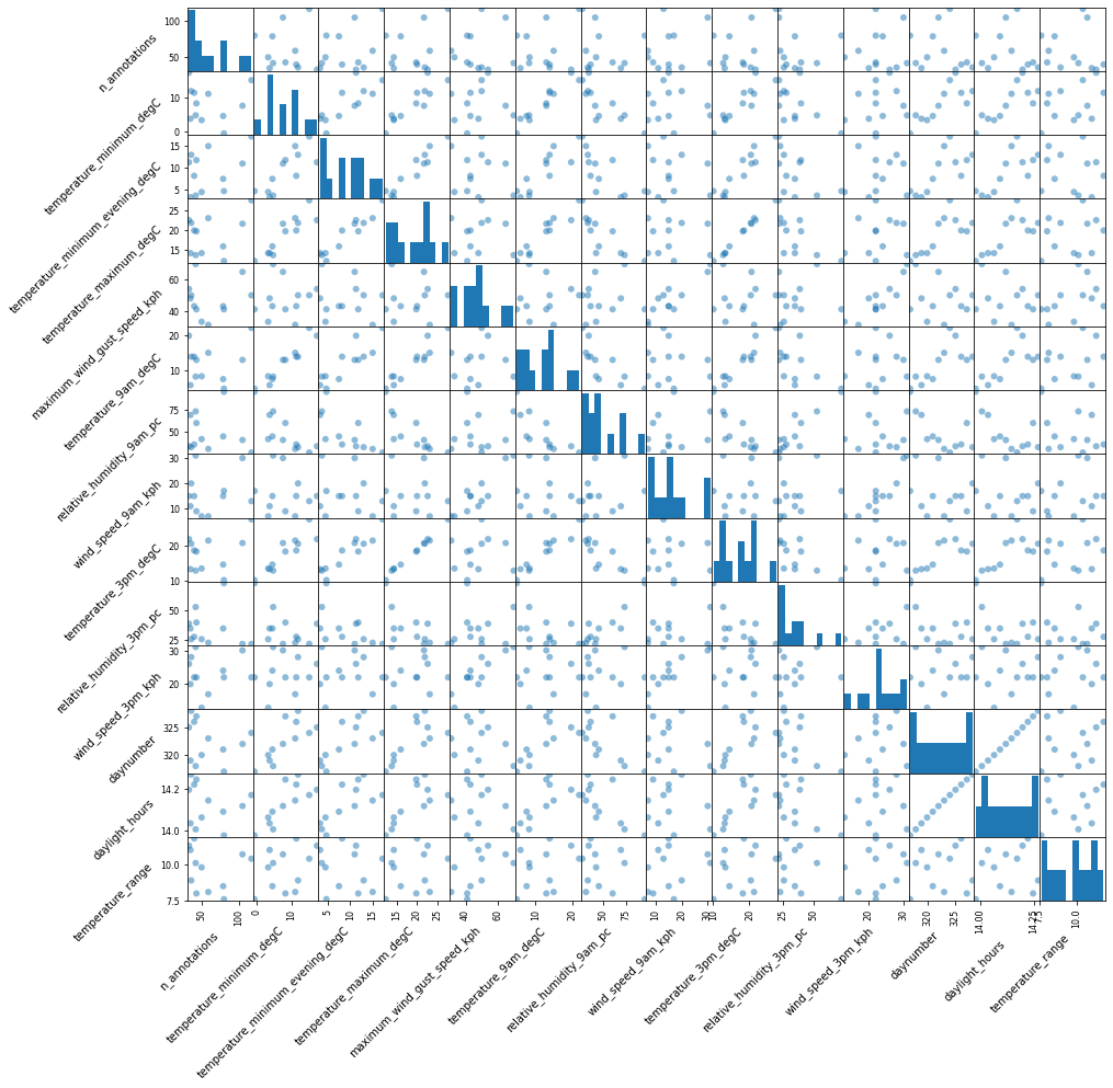
Some of these look like they are correlated, so we should remove them from the list of covariates. We start by finding the pearson correlation between each of the varibles.

Note that the below dataframe has ones on the leading diagonal. Strictly speaking, these should be zeros (but leaving them as ones happens to be more convenient in this case).

correlation_p_vals = maelstrom_df[covariates].corr(
    method=lambda x, y: sp.stats.pearsonr(x, y)[1]
)

n_annotations_corr = maelstrom_df[covariates].corrwith(
    maelstrom_df["n_annotations"]
)

correlation_p_vals

	temperature_minimum_degC	temperature_minimum_evening_degC	temperature_maximum_degC	maximum_wind_gust_speed_kph	temperature_9am_degC	relative_humidity_9am_pc	wind_speed_9am_kph	temperature_3pm_degC	relative_humidity_3pm_pc	wind_speed_3pm_kph	daynumber	daylight_hours	temperature_range
temperature_minimum_degC	1.000000	0.002116	7.228477e-05	0.726410	0.000001	0.002227	0.765180	5.734440e-05	0.061840	0.583986	2.849026e-03	2.297827e-03	0.200886
temperature_minimum_evening_degC	0.002116	1.000000	1.477610e-06	0.773894	0.000269	0.009102	0.598260	1.022308e-05	0.059156	0.843996	8.241975e-03	7.022097e-03	0.768792
temperature_maximum_degC	0.000072	0.000001	1.000000e+00	0.886576	0.000003	0.001713	0.766278	1.321696e-11	0.019935	0.710210	6.060147e-03	4.804292e-03	0.518073
maximum_wind_gust_speed_kph	0.726410	0.773894	8.865758e-01	1.000000	0.765853	0.708056	0.000074	7.875770e-01	0.711903	0.000115	7.235197e-01	7.176197e-01	0.134835
temperature_9am_degC	0.000001	0.000269	2.677875e-06	0.765853	1.000000	0.003710	0.752917	1.057270e-06	0.069890	0.712510	9.914545e-03	8.194690e-03	0.306516
relative_humidity_9am_pc	0.002227	0.009102	1.712610e-03	0.708056	0.003710	1.000000	0.518422	1.337258e-03	0.000111	0.789428	1.408504e-02	1.071846e-02	0.290696
wind_speed_9am_kph	0.765180	0.598260	7.662779e-01	0.000074	0.752917	0.518422	1.000000	8.017529e-01	0.494823	0.000090	5.306412e-01	5.172520e-01	0.463215
temperature_3pm_degC	0.000057	0.000010	1.321696e-11	0.787577	0.000001	0.001337	0.801753	1.000000e+00	0.015457	0.700807	9.167460e-03	7.319337e-03	0.405187
relative_humidity_3pm_pc	0.061840	0.059156	1.993542e-02	0.711903	0.069890	0.000111	0.494823	1.545673e-02	1.000000	0.566386	6.486753e-02	5.388663e-02	0.244309
wind_speed_3pm_kph	0.583986	0.843996	7.102099e-01	0.000115	0.712510	0.789428	0.000090	7.008068e-01	0.566386	1.000000	7.355078e-01	7.546994e-01	0.552350
daynumber	0.002849	0.008242	6.060147e-03	0.723520	0.009915	0.014085	0.530641	9.167460e-03	0.064868	0.735508	1.000000e+00	2.993460e-16	0.750526
daylight_hours	0.002298	0.007022	4.804292e-03	0.717620	0.008195	0.010718	0.517252	7.319337e-03	0.053887	0.754699	2.993460e-16	1.000000e+00	0.723849
temperature_range	0.200886	0.768792	5.180730e-01	0.134835	0.306516	0.290696	0.463215	4.051872e-01	0.244309	0.552350	7.505260e-01	7.238494e-01	1.000000

We remove correlated variables in a greedy fashion, recursively selecting the most significantly correlated pair of variables, and removing the one which is not as well correlated with “n_annotations”. We’ll use a stringent p-value cutoff of 0.001 to make sure we don’t throw away any important variables.

def greedy_variate_removal(correlation_p_vals, p_cutoff, scores):
    r, c = divmod(np.argmin(correlation_p_vals), len(correlation_p_vals))

    if correlation_p_vals.iloc[r, c] >= p_cutoff:  # We're done!
        return correlation_p_vals

    drop_label = correlation_p_vals.index[
        [r, c][
            scores[correlation_p_vals.index[[r, c]]].argmin()
        ]
    ]
    correlation_p_vals = correlation_p_vals.drop(index=drop_label)
    correlation_p_vals.drop(columns=drop_label, inplace=True)

    return greedy_variate_removal(correlation_p_vals, p_cutoff, scores)


correlation_p_vals = greedy_variate_removal(
    correlation_p_vals, 0.001, n_annotations_corr
)
filtered_covariates = list(correlation_p_vals.index)
correlation_p_vals

	temperature_minimum_degC	temperature_minimum_evening_degC	relative_humidity_9am_pc	wind_speed_9am_kph	daylight_hours	temperature_range
temperature_minimum_degC	1.000000	0.002116	0.002227	0.765180	0.002298	0.200886
temperature_minimum_evening_degC	0.002116	1.000000	0.009102	0.598260	0.007022	0.768792
relative_humidity_9am_pc	0.002227	0.009102	1.000000	0.518422	0.010718	0.290696
wind_speed_9am_kph	0.765180	0.598260	0.518422	1.000000	0.517252	0.463215
daylight_hours	0.002298	0.007022	0.010718	0.517252	1.000000	0.723849
temperature_range	0.200886	0.768792	0.290696	0.463215	0.723849	1.000000

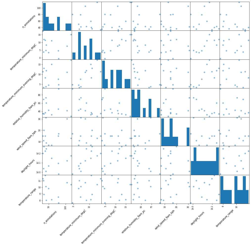
With this new filtered list of covariates, we again plot the pairs to make sure that everything looks nice and uncorrelated.

grr = pd.plotting.scatter_matrix(
    maelstrom_df[["n_annotations", *filtered_covariates]],
    marker="o",
    figsize=(15, 15),
)
for ax in grr[-1, :]:
    ax.set_xlabel(ax.get_xlabel(), rotation=45, ha="right")
for ax in grr[:, 0]:
    ax.set_ylabel(ax.get_ylabel(), rotation=45, ha="right")

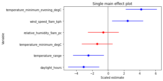
Fitting a Poisson GLM of n_annotations vs. each covariate individually, and plotting the effect:

pois = sm.families.Poisson()

tvalues = []
pvalues = []
for covariate in filtered_covariates:
    mod = smf.glm(
        f"n_annotations ~ {covariate}",
        data=maelstrom_df,
        family=pois,
        exposure=maelstrom_df["exposures"],
    )
    res = mod.fit()
    tvalues.append(res.tvalues[1])
    pvalues.append(res.pvalues[1])

tvalues = np.array(tvalues)
pvalues = np.array(pvalues)

ordering = np.argsort(tvalues)
coloring = np.array(["r", "b"])[(pvalues[ordering] < 0.05).astype("u1")]

fig = plt.figure()
ax = fig.add_subplot(
    111,
    title="Single main effect plot",
    xlabel="Scaled estimate",
    ylabel="Variable",
)
ax.axvline(0, c="gray")
ax.hlines(
    np.array(filtered_covariates)[ordering],
    tvalues[ordering] - 1.96,
    tvalues[ordering] + 1.96,
    color=coloring
)
p = ax.scatter(
    tvalues[ordering],
    np.array(filtered_covariates)[ordering],
    color=coloring
)

significant_single_effect_variables = set(np.array(filtered_covariates)[pvalues < 0.05])
print("Significant single-effect variables:", *significant_single_effect_variables, sep="\n  - ")

Significant single-effect variables:
  - daylight_hours
  - temperature_minimum_evening_degC
  - temperature_range
  - wind_speed_9am_kph

Fitting a Poisson GLM of n_annotations vs. all of the covariates, and plotting the effect:

mod = smf.glm(
    "n_annotations ~ " + " + ".join(filtered_covariates),
    data=maelstrom_df,
    family=pois,
    exposure=maelstrom_df["exposures"],
)
res = mod.fit()
print(res.summary())
print(f"res.aic={res.aic}")

ordering = np.argsort(res.tvalues)
coloring = np.array(["r", "b"])[
    (res.pvalues[ordering] < 0.05).astype("u1")
]

fig = plt.figure()
ax = fig.add_subplot(
    111,
    xlabel="Scaled estimate",
    ylabel="Variable",
)
ax.axvline(0, c="gray")
ax.hlines(
    res.tvalues.index[ordering],
    res.tvalues[ordering] - 1.96,
    res.tvalues[ordering] + 1.96,
    color=coloring,
)
p = ax.scatter(res.tvalues[ordering], res.tvalues.index[ordering], color=coloring)

significant_mixed_effect_variables = set(res.tvalues.index[res.pvalues < 0.05])

print("\nSignificant mixed-effect variables:", *significant_mixed_effect_variables, sep="\n  - ")

                 Generalized Linear Model Regression Results
==============================================================================
Dep. Variable:          n_annotations   No. Observations:                   12
Model:                            GLM   Df Residuals:                        5
Model Family:                 Poisson   Df Model:                            6
Link Function:                    log   Scale:                          1.0000
Method:                          IRLS   Log-Likelihood:                -47.274
Date:                Mon, 09 Aug 2021   Deviance:                       24.473
Time:                        14:47:53   Pearson chi2:                     24.2
No. Iterations:                     4
Covariance Type:            nonrobust
====================================================================================================
                                       coef    std err          z      P>|z|      [0.025      0.975]
----------------------------------------------------------------------------------------------------
Intercept                           41.3617     11.516      3.592      0.000      18.790      63.933
temperature_minimum_degC            -0.1297      0.025     -5.230      0.000      -0.178      -0.081
temperature_minimum_evening_degC     0.1897      0.022      8.543      0.000       0.146       0.233
relative_humidity_9am_pc            -0.0017      0.004     -0.468      0.640      -0.009       0.005
wind_speed_9am_kph                   0.0062      0.006      1.120      0.263      -0.005       0.017
daylight_hours                      -3.1266      0.806     -3.881      0.000      -4.705      -1.548
temperature_range                    0.1548      0.052      3.000      0.003       0.054       0.256
====================================================================================================
res.aic=108.54753196329011

Significant mixed-effect variables:
  - temperature_minimum_degC
  - daylight_hours
  - temperature_minimum_evening_degC
  - Intercept
  - temperature_range

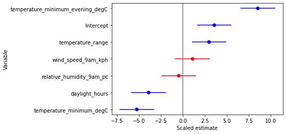
From the above plot, we can see that some of the variables do not have a significant effect on “n_annotations”. So let’s remove them and see if we get a better model.

sig_eff_variables = list(significant_mixed_effect_variables - {"Intercept"})

mod = smf.glm(
    "n_annotations ~ " + " + ".join(sig_eff_variables),
    data=maelstrom_df,
    family=pois,
    exposure=maelstrom_df["exposures"],
)
res = mod.fit()
print(res.summary())
print(f"res.aic={res.aic}")

ordering = np.argsort(res.tvalues)
coloring = np.array(["r", "b"])[
    (res.pvalues[ordering] < 0.05).astype("u1")
]

fig = plt.figure()
ax = fig.add_subplot(
    111,
    xlabel="Scaled estimate",
    ylabel="Variable",
)
ax.axvline(0, c="gray")
ax.hlines(
    res.tvalues.index[ordering],
    res.tvalues[ordering] - 1.96,
    res.tvalues[ordering] + 1.96,
    color=coloring,
)
p = ax.scatter(res.tvalues[ordering], res.tvalues.index[ordering], color=coloring)

                 Generalized Linear Model Regression Results
==============================================================================
Dep. Variable:          n_annotations   No. Observations:                   12
Model:                            GLM   Df Residuals:                        7
Model Family:                 Poisson   Df Model:                            4
Link Function:                    log   Scale:                          1.0000
Method:                          IRLS   Log-Likelihood:                -47.915
Date:                Mon, 09 Aug 2021   Deviance:                       25.756
Time:                        14:47:53   Pearson chi2:                     25.3
No. Iterations:                     4
Covariance Type:            nonrobust
====================================================================================================
                                       coef    std err          z      P>|z|      [0.025      0.975]
----------------------------------------------------------------------------------------------------
Intercept                           39.6614     10.961      3.618      0.000      18.178      61.144
temperature_minimum_degC            -0.1381      0.024     -5.790      0.000      -0.185      -0.091
temperature_minimum_evening_degC     0.1997      0.020     10.108      0.000       0.161       0.238
daylight_hours                      -3.0297      0.775     -3.909      0.000      -4.549      -1.511
temperature_range                    0.1882      0.041      4.562      0.000       0.107       0.269
====================================================================================================
res.aic=105.83037074639384

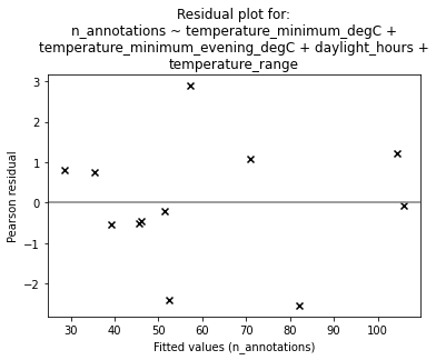
Removing the variables from the model lowered AIC, meaning that not much information was lost, while reducing the risk of overfitting. We will proceed with this model.

To check that nothing strange is going on, we can plot the residuals:

fig = plt.figure()
ax = fig.add_subplot(
    111,
    title="Residual plot for:\n" + "\n".join(textwrap.wrap(mod.formula, width=55)),
    ylabel="Pearson residual",
    xlabel="Fitted values (n_annotations)",
)

ax.axhline(0, c="gray")
p = ax.scatter(res.fittedvalues, res.resid_pearson, marker="x", c="k")

Finally, we can combine the summary abundance/activity plots from above, this time including the predicted values for “n_annotations” (and confidence interval) into the maelstrom plot.

prediction = res.get_prediction()

# Set up figure
fig = plt.figure(
    figsize=(7.5, 5.2),
    tight_layout=True,
)
title_y = 0.87
title_fontdict = {"fontweight": "bold"}

# Define each subplot
# General summary plot
ax1 = fig.add_subplot(
    221,
    xlabel="Day Number",
    ylabel="Number of annotations",
)
ax1.set_title(
    " (a)", fontdict=title_fontdict, loc="left", y=title_y
)
# Twilight plot
ax2 = fig.add_subplot(
    222,
    xlabel="Twilight durations since sunset",
)
ax2.set_title(
    " (b)", fontdict=title_fontdict, loc="left", y=title_y
)
# Maelstrom plot with temperatures
ax3 = fig.add_subplot(
    212,
    xlabel="Day Number",
    ylabel="Number of annotations\nDuring twilight",
)
ax3.set_title(
    " (c)", fontdict=title_fontdict, loc="left", y=title_y
)

# Actual plotting
# General summary plot
plot_activity_levels_summary(
    df,
    ax1,
    x_column="daynumber",
    bin_width=10 / 1440,   # 10 minutes
    c="k",
    lw=0.75,
)

# Twilight plot
plot_activity_levels_summary(
    df,
    ax2,
    x_column="within_twilight",
    bin_width=0.1,   # 10th of twilight duration
    c="k",
    lw=0.75,
)
twilight_vspan = ax2.axvspan(
    0, 1, alpha=0.3, label="Evening twilight"
)

# Maelstrom plot with temperatures
plot_maelstroms_with_temperature(
    maelstrom_df,
    ax3,
    maelstrom_kwargs=dict(
        c="k",
        lw=3,
    ),
)

# Model prediction
ax3.plot(
    maelstrom_df["daynumber"],
    prediction.predicted_mean * maelstrom_df["exposures"],
    color="g",
    alpha=0.7,
    linestyle="dotted",
)
conf_int = prediction.conf_int()
ax3.fill_between(
    maelstrom_df["daynumber"],
    conf_int[:, 0] * maelstrom_df["exposures"],
    conf_int[:, 1] * maelstrom_df["exposures"],
    color="g",
    alpha=0.25,
    linestyle="dotted",
)

# Force x-axis ticks to be integers to make it prettier
for ax in fig.axes:
    ax.xaxis.set_major_locator(MaxNLocator(integer=True))

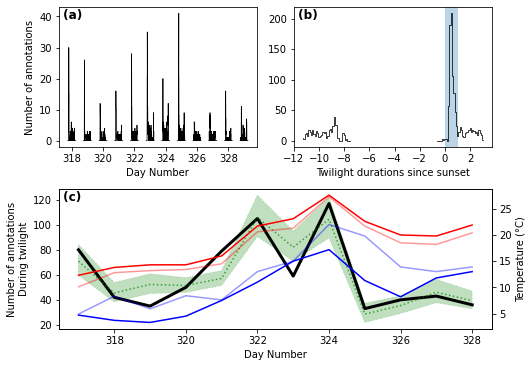
fig.savefig("activity_levels_figure.pdf", dpi=600.0, pad_inches=0.0)